Tutorial: Import Data into Excel, and Create a Data Model

Abstract: This is the first tutorial in a series designed to get you acquainted and comfortable using Excel and its built-in data mash-up and analysis features. These tutorials build and refine an Excel workbook from scratch, build a data model, then create amazing interactive reports using Power View. The tutorials are designed to demonstrate Microsoft Business Intelligence features and capabilities in Excel, PivotTables, Power Pivot, and Power View.

In these tutorials you learn how to import and explore data in Excel, build and refine a data model using Power Pivot, and create interactive reports with Power View that you can publish, protect, and share.

The tutorials in this series are the following:

1. Import Data into Excel 2016, and Create a Data Model
2. Extend Data Model relationships using Excel, Power Pivot, and DAX
3. Create Map-based Power View Reports
4. Incorporate Internet Data, and Set Power View Report Defaults
5. Power Pivot Help
6. Create Amazing Power View Reports - Part 2

In this tutorial, you start with a blank Excel workbook.

The sections in this tutorial are the following:

• Import data from a database
• Import data from a spreadsheet
• Import data using copy and paste
• Create a relationship between imported data
• Checkpoint and Quiz

At the end of this tutorial is a quiz you can take to test your learning.

This tutorial series uses data describing Olympic Medals, hosting countries, and various Olympic sporting events. We suggest you go through each tutorial in order.

Import data from a database

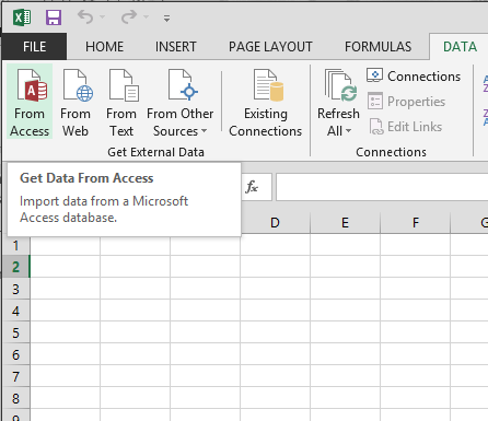
We start this tutorial with a blank workbook. The goal in this section is to connect to an external data source, and import that data into Excel for further analysis.

Let’s start by downloading some data from the Internet. The data describes Olympic Medals, and is a Microsoft Access database.

1. Click the following links to download files we use during this tutorial series. Download each of the four files to a location that’s easily accessible, such as Downloads or My Documents, or to a new folder you create:
   >OlympicMedals.accdb Access database
   >OlympicSports.xlsx Excel workbook
   >Population.xlsx Excel workbook
   >DiscImage_table.xlsx Excel workbook
2. In Excel, open a blank workbook.
3. Click DATA > Get External Data > From Access. The ribbon adjusts dynamically based on the width of your workbook, so the commands on your ribbon may look slightly different from the following screens. The first screen shows the ribbon when a workbook is wide, the second image shows a workbook that has been resized to take up only a portion of the screen.

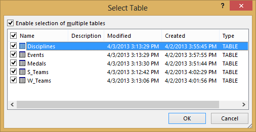Select table window" />

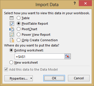
Note: Notice the checkbox at the bottom of the window that allows you to Add this data to the Data Model, shown in the following screen. A Data Model is created automatically when you import or work with two or more tables simultaneously. A Data Model integrates the tables, enabling extensive analysis using PivotTables, Power Pivot, and Power View. When you import tables from a database, the existing database relationships between those tables is used to create the Data Model in Excel. The Data Model is transparent in Excel, but you can view and modify it directly using the Power Pivot add-in. The Data Model is discussed in more detail later in this tutorial.

Select the PivotTable Report option, which imports the tables into Excel and prepares a PivotTable for analyzing the imported tables, and click OK.

With the data imported into Excel, and the Data Model automatically created, you’re ready to explore the data.

Explore data using a PivotTable

Exploring imported data is easy using a PivotTable. In a PivotTable, you drag fields (similar to columns in Excel) from tables (like the tables you just imported from the Access database) into different areas of the PivotTable to adjust how it presents your data. A PivotTable has four areas: FILTERS, COLUMNS, ROWS, and VALUES.

It might take some experimenting to determine which area a field should be dragged to. You can drag as many or few fields from your tables as you like, until the PivotTable presents your data how you want to see it. Feel free to explore by dragging fields into different areas of the PivotTable; the underlying data is not affected when you arrange fields in a PivotTable.

Let’s explore the Olympic Medals data in the PivotTable, starting with Olympic medalists organized by discipline, medal type, and the athlete’s country or region.

1. In PivotTable Fields, expand the Medals table by clicking the arrow beside it. Find the NOC_CountryRegion field in the expanded Medals table, and drag it to the COLUMNS area. NOC stands for National Olympic Committees, which is the organizational unit for a country or region.
2. Next, from the Disciplines table, drag Discipline to the ROWS area.
3. Let’s filter Disciplines to display only five sports: Archery, Diving, Fencing, Figure Skating, and Speed Skating. You can do this from within the PivotTable Fields area, or from the Row Labels filter in the PivotTable itself.
   1. Click anywhere in the PivotTable to ensure the Excel PivotTable is selected. In the PivotTable Fields list, where the Disciplines table is expanded, hover over its Discipline field and a dropdown arrow appears to the right of the field. Click the dropdown, click (Select All)to remove all selections, then scroll down and select Archery, Diving, Fencing, Figure Skating, and Speed Skating. Click OK.
   2. Or, in the Row Labels section of the PivotTable, click the dropdown next to Row Labels in the PivotTable, click (Select All) to remove all selections, then scroll down and select Archery, Diving, Fencing, Figure Skating, and Speed Skating. Click OK.
4. In PivotTable Fields, from the Medals table, drag Medal to the VALUES area. Since Values must be numeric, Excel automatically changes Medal to Count of Medal.
5. From the Medals table, select Medal again and drag it into the FILTERS area.
6. Let’s filter the PivotTable to display only those countries or regions with more than 90 total medals. Here’s how.
   1. In the PivotTable, click the dropdown to the right of Column Labels.
   2. Select Value Filters and select Greater Than….
   3. Type 90 in the last field (on the right). Click OK.
      

      Your PivotTable looks like the following screen.

      

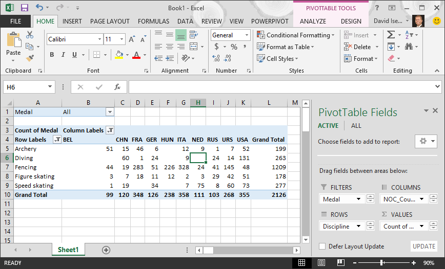
      With little effort, you now have a basic PivotTable that includes fields from three different tables. What made this task so simple were the pre-existing relationships among the tables. Because table relationships existed in the source database, and because you imported all the tables in a single operation, Excel could recreate those table relationships in its Data Model.

      But what if your data originates from different sources, or is imported at a later time? Typically, you can create relationships with new data based on matching columns. In the next step, you import additional tables, and learn how to create new relationships.

      Import data from a spreadsheet

      Now let’s import data from another source, this time from an existing workbook, then specify the relationships between our existing data and the new data. Relationships let you analyze collections of data in Excel, and create interesting and immersive visualizations from the data you import.

      Let’s start by creating a blank worksheet, then import data from an Excel workbook.

      1. Insert a new Excel worksheet, and name it Sports.
      2. Browse to the folder that contains the downloaded sample data files, and open OlympicSports.xlsx.
      3. Select and copy the data in Sheet1. If you select a cell with data, such as cell A1, you can press Ctrl + A to select all adjacent data. Close the OlympicSports.xlsx workbook.
      4. On the Sports worksheet, place your cursor in cell A1 and paste the data.
      5. With the data still highlighted, press Ctrl + T to format the data as a table. You can also format the data as a table from the ribbon by selecting HOME > Format as Table. Since the data has headers, select My table has headers in the Create Table window that appears, as shown here.

      

      

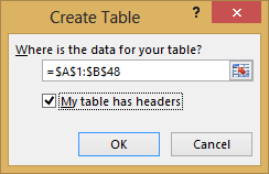
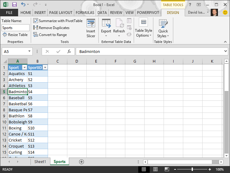
      Formatting the data as a table has many advantages. You can assign a name to a table, which makes it easy to identify. You can also establish relationships between tables, enabling exploration and analysis in PivotTables, Power Pivot, and Power View. Name the table. In TABLE TOOLS > DESIGN > Properties, locate the Table Name field and type Sports. The workbook looks like the following screen.
      

      Import data using copy and paste

      Now that we’ve imported data from an Excel workbook, let’s import data from a table we find on a web page, or any other source from which we can copy and paste into Excel. In the following steps, you add the Olympic host cities from a table.

      1. Insert a new Excel worksheet, and name it Hosts.
      2. Select and copy the following table, including the table headers.

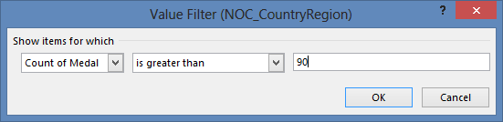
      NOC_CountryRegion